Sample fMRI Event Design Analysis using FSL

Background

• To complete this tutorial you will need:
  1. FSL installed on your computer (included with Lin4Neuro).
  2. The sample dataset that includes the fMRI data (in NIfTI format) and timing files. Lin4Neuro includes this in the home folder "tutorial".

About the sample dataset

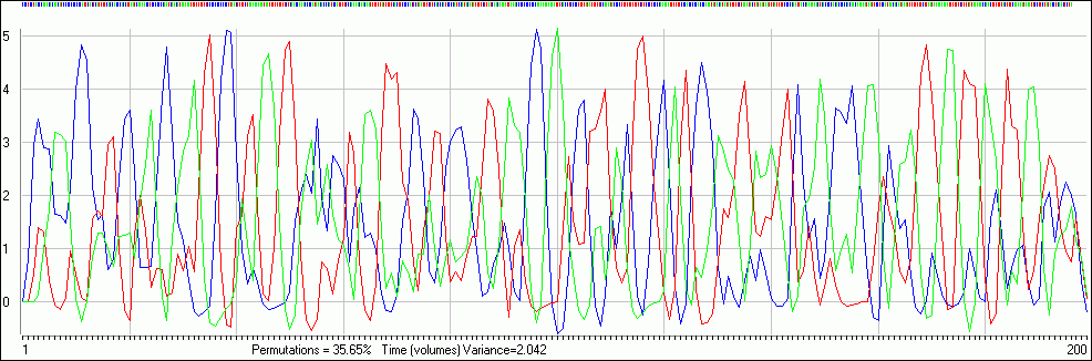
This was a simple finger tapping task. The screen rapidly flashed with an arrow (< or >). When the arrow pointed right (>) they were intstructed to tap their right index finger, and when it pointed left (<) they were requested to push their left index finger. These events repeated for the whole scanning session (302 volumes, about 10 minutes). The MRI scanner actually recorded 304 volumes, but automatically discarded the first two (as these have T1 effects), with all event onset times referring to the start of the first stored volume. The onsets of the tasks are recorded in the text files (LEVent.tab,REvent.tab). The image below shows the three event types (left, right arrow) as marks at the top of the image (with red and green indicating the stimuli types). The colored lines show the expected HRF response.

FSL single subject data processing

FSL's tabs
1. From the command line, type "cd ~/tutorial" to change to the folder with the tutorial data. Next start FSL by typing 'fsl &'.
2. By typing fsl, a user interface (the one with a fossil fish on its top, the logo for 'FSL') appears. This interface contains several options, for this tutorial we will use BET and FEAT.
3. Creating a scalp-stripped MRI scan: from the main FSL menu, press "BET brain extraction", press the folder button next to input image and select the T1 image (T1s005) and press go. This will create the image T1s005_brain as output.
   • Advanced notes:
   • For this tutorial we will use our high resolution T1-image to aid the normalization of our low-resolution fMRI data. This is optional, but often results in better statistics across a group of people. One problem is that the T1 image shows a lot of non-brain tissue (neck, eyeballs, fat of scalp, etc). However, we really want our normalization to be based on the brain shape, rather than trying to match these other features. Therefore we will use BET to scalp strip.
   • It is typically important to check that the brain is accurately extracted - to do this open the resulting output with MRIcron or FSLview. If the extracted image is inaccurate, you can can adjust the "Fractional intensity estimate" with BET. For example, if the output image includes too much tissue (e.g. neck or eyes included in the output) make this value larger (e.g. 0.6), whereas if the output removes too much gray matter make this value smaller (e.g. 0.4). Another way you can adjust this is to open the source image with MRIcron and choose Draw/Advanced/CropEdges (if you do not see the drawing menu, choose Help/Preferences and select 'Show drawing menus", and adjust the values so that the only the brain is visible (if too much neck is visible, BET will have a poor starting estimate) and then press 'Save Cropped'. Use this new cropped image as your input for BET.
4. Start FEAT: From the main FSL menu, press "FEAT FMRI analysis" This will open the Feat interface. (The following steps are described for use in FEAT version 5.98)The feat interface has two top buttons. The following analysis is a first level analysis (within one single subject).The FEAT interface five tabs across the top portion of the screen, oriented in a horizontal line. The fmri analysis can be set by defining the parameters within each one of those buttons, in a left to right order: Data, Pre-stats, Stats, Post-stats, and Registration.
5. Data Tab: - Number of analysis is set to one. - Press select 4D data. Browse to the folder in which the 4D data file is stored and select the corresponding file (e.g. fmrievents008) After selecting the 4D file, the number of volumes will automatically be displayed. In our case 302. - enter the TR. In our case 1.92. Set the delete volumes to 0. Leave the high pass filter cutoff at 100 s. You can set the output directory: you must be able to write to this directory. If you leave it blank, it will write the results in the same folder where the 4D data is. FEAT write the results in a folder called "4Ddataname.feat". In our case fmrievents008.feat. If you re-run the analysis, it will create a second folder called fmrievents008.feat+, and so on.
6. Pre-stats Tab: - Optional: slice timing correction could be set to regular up (0,1,2...n-1). Keep the default Motion correction (FMRIB's Linear Image Registration Tool - MCFLIRT). Keep "Brain Extraction" checked. Set "Spatial smoothing FWHM" set to 8mm (between x2-x3 the raw resolution of the functional imaging). Lets keep Intensity Normalization" (equivalent to Grand Mean Scaling) unchecked. Keep "Temporal filtering Highpass" checked.
7. Stats Tab: The onsets timings of our design is intricate so press the 'Full Model Setup' button. - Clicking full model setup opens a "General Linear Model" interface. Within this interface, follow the steps: - The number of original EV (original EVS - explanatory variables, or simply put: conditions) is set to 2, because we are interested in the response to the "left" and "right" conditions. - Each EV is setup separately. - The basic shape of the wave form that describes the stimulus that we wish to model is defined by a custom file expliciting the time in seconds of the onset of the stimulus, how much time (also in seconds) the stimulus last, and the value of the input. This requires a text file containing a matrix under which the columns are the variables stated above (i.e., first one time of onset, second one the duration, and the thrid one the intensity) and the rows represent the stimuli.
   
• Setting Up Conditions: This is set as follows: set the "Number of original EVs" to 2. This will create two sub-Tabs in the EVs tab ('1','2': one for each condition). For the '1' tab, set the EV name to "L" and choose the 'Custom (3 column format)' option from the 'Basic Shape' pull-down menu, finally set the filename (press the folder icon to browse for the filename) to LEvent.tab". For the '2' tab, set the EV name to "R" and choose the 'Custom (3 column format)' option from the 'Basic Shape' pull-down menu, finally set the filename (press the folder icon to browse for the filename) to "REvent.tab".
  • Setting Up contrasts: Once these parameters have been entered click on 'Contrasts & F-tests' tab. In theory, we could create quite a few statistical comparisons, for example, here are five possible contrasts of interest:
  • OC1: Find what is active for left motor presses: title= left>, EV1= 1, EV2= 0
  • OC2: Find regions more active for left than right motor: title= left>right, EV1= 1, EV2= -1
  • OC3: Find what is active for right motor presses: title= right>, EV1= 0, EV2= 1
  • OC4: Find regions more active for right than left motor: title= left>right, EV1= -1, EV2= 1
  • OC5: Find regions more active for any motor activity title= motor>rest, EV1= 1, EV2= 1
• Alternatively, we could only look at our two favorite conditions (left > right and right > left).
• Press Done to continue.
8. Post_stats Tab: Keep all the defaults.
9. Registration Tab: We have a structural image for this participant, so check the "Main structural image" box and click the folder icon to set this to point to our scalp stripped image (T1s005_brain) That we created earlier. Make sure that both the "main structural image" and "standard space" normalizations use 12 DOF (12 parameters: rotation, zoom, shear, translation in 3 dimensions) - this is often not set by default, but works much better.
10. Press the 'Go' button on the bottom left. Press the 'Go' button on the bottom left. FEAT will launch a web page that shows you the status of the analysis and eventually displays the results.