Creating 3D ROIs with MRIcro

Introduction

Note: The features described here will be introduced with MRIcro 1.36 or later.

Regions of Interest (ROIs) are a way of marking specific parts of an image. For example, an ROI could define the location and extent of a stroke in a scan of a brain, or define the location of the temporal lobe in a healthy adult. ROIs have multiple uses: for work with neurological patients, ROIs can map the location and extent of a lesion. In addition, ROIs can be used to understand the role of a specific area of the healthy brain when applied to functional brain images (images that indirectly map brain activity). Traditionally, ROIs are created by mapping the regions on each and every 2D slice of a 3D volume using a pen tool (e.g. as described in my MRIcro tutorial). However, creating ROIs in this manner is usually quite tedious. This page describes how the latest versions of MRIcro (1.36 and later) can create 3D regions of interest in a few simple steps. These new tools can be combined with MRIcro's traditional tools to quickly speed the drawing of ROIs.

Getting Started

The latest versions of MRIcro includes two new tools in the 'Region of Interest' panel:

3D Painting Tool

The 3D painting tool allows you to generate a ROI by selecting a contiguous cluster of voxels defined by the intensity of the underlying image; for example, you could quickly create a ROI that selects the gray matter of a brain without including the white matter. When you click on the tool's button, a new window appears with a number of controls that define the properties of the ROI. Simply double click on the image at any location to draw a ROI around that location. Here is a short overview of the controls:

Origin: defines the starting (seed) location for the ROI. You can double-click on the image to select a new origin.
Difference from origin: Maximum image intensity difference between seed and any other voxel included in the ROI. For example, if set to zero, only voxels with exactly the same brightness as the origin will be selected. On the other hand, if this is set to 10, voxels that are slightly brighter or darker than the origin will be included.
Difference at edge: Maximum brightness difference between adjacent voxels for a voxel to be included in the ROI. A voxel must satisfy both the difference from origin and the difference at edge constraints to be included.
ROI radius (mm): Maximum radius of the ROI; voxels further away than this from the origin will not be included in the cluster.
Erode/dilate cycles: This control allows you to only include regions that are strongly connected to the origin. This can prevent the ROI from bleeding into unwanted regions.
Append to current ROI: If a ROI is already open, you will be able to click on this button to choose whether the new ROI is added (appended), subtracted (deleted) or constrained by the previous ROI. These options are illustrated on the right: the red bar indicates the location of the original ROI, with the new ROI shown as green.

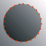
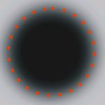
Note that the edge of the boundary can be defined as the difference from origin, the difference at the edge or a combination of these two constraints. You will want to vary your usage of these based on your image. On the right I show two examples to illustrate this decision. Assume you want to mark the edge shown by orange dots in each figure. For the global gradient (often seen near the edge of the field of view in many MRI scans) the 'difference from origin' is a poor estimate of the edge, while the 'difference at edge' is a better estimate. For this image, you would want to set 'difference at origin' to 255, and initially set the 'difference from edge' to a low value and increase the 'difference from edge' until you select your region. The opposite technique should be used for the 'blurred edge' example, where the difference at edge is a poorer estimate for the desired edge than the difference from the (centrally placed) origin.

Also note that this tool makes it easy to create a sphere. Simply set large "Difference from origin" and "Difference at edge" values, leaving the Radius as the only constraint.

Left: global gradient,
Right: blurred edge

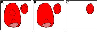
3D Bubble Fill

Sometimes, you will find that a region of interest contains a "bubble" of unincluded voxels. These are tedious to fill in by hand, and this tool removes them instantly. It is also useful when you want to delete a whole connected ROI, for example if the automatic selection process has "bled" across a narrow bridge into an irrelevant region, and you have removed the bridge by hand.

Consider the image with two 3D ROIs shown on the right (A). Note that each object has a bubble trapped inside. Ctrl-Clicking with the bubble tool anywhere (except inside the bubble) on the large object will fill its bubble, resulting in B. Note that the pocket at the bottom of the object is not affected: it is open to the outside so is not a bubble. Also, note that the smaller ROI is not affected: it is an independent object.

Ctrl-Shift-clicking on any ROI deletes the entire 3D object, for example shift+clicking on the large object from A results in C. Again, the small object is not affected, as it is not contiguous with the large object (so it is treated as a separate object).

Technical Notes

The current 3D ROI tools in MRIcro are pretty primitive. If I had the time, I would certainly investigate more sophisticated techniques. A number of techniques would be very useful, and would be particularly powerful if used together:

Automated segmentation into regions following normalization. Automated software can 'normalize' brains to stereotaxic space (warping the overall shape and size of an individuals brain to a standard space). Once this is achieved, it should be fairly straight forward to identify regions based on a priori priniciples (e.g. the basal ganglia will be approximately in the same location across individuals, and it will appear darker in T1 scans than the surrounding white matter). The gray/white matter segmentation of SPM suggests a good starting point for this approach, and it could certainly be applied more specifically to new problems.
Morphological identification of regions. The tools I use are based simply on the relative brightness. Mathematical models of these images as morphological maps (e.g. consider bright areas as representing higher ground than dark areas, and different ROIs as competing bodies of liquid filling the terrain). Nice examples of these techniques are shown at www.mmorph.com.
Some pioneers have described fairly automated tools for identifying cortical landmarks (gyri and sulci). For example, see Caunce and Taylor (2001, Building 3D sulcal models using local geometry. Medical Image Analysis 5, 69-80). Paul THompson and colleagues at UCLA have also done some nice work on this topic.