Important note: By default, MRIcron has the lesion drawing tools switched off. To turn on the lesion drawing features of MRIcron, select Help/Preferences and make sure the "Show drawing menu and tools" checkbox is selected.

Flash videos, scripts and sample data are available to help users master these techniques.

MRIcron is designed to relate lesion location to behavioral performance. For example, it can help identify brain regions that are crucial to language production. To conduct an analysis, we will need to conduct four steps:

1. Lesion Mapping: For each individual, we need to map the extent of brain injury.
2. Specify design: We need to design our experiment, creating a spreadsheet that links each individual's lesion map to their performance
3. Compute results: We need to conduct a voxelwise statistical analysis.
4. Viewing results: We need to interpret the results.

1. A copy of MRIcron: the version will include a folder named 'example\lesions' with the sample dataset described here.
2. A copy of NPM (installed when you install MRIcron)

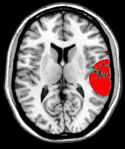
Right: A sample lesion map (9.voi) overlayed ontop of the ch2 template showing injury to the left temporal lobe. To view this map, launch MRIcron and choose File/Template/Ch2, then choose Overlay/Add... and choose the image 9.voi included with the sample dataset.

Lesion Mapping

MRIcron provides simple tools for drawing a region of brain injury. However, it is crucial that all of our lesion maps are drawn with the same image dimensions and orientation. Therefore, we should either draw all the lesions on a standard template (e.g. File/OpenTemplates/CH2), or we need to first normalize all the scans so they are coregistered and then open each scan using File/Open.

1. Launch MRIcron and open your scan (File/Open or File/OpenTemplate)
2. Select your drawing tool (these are listed at the bottom of the Draw menu, e.g. the 'Pen' tool).
3. Draw your region - for example if you use the 'Autoclose Pen' tool, simply click and draw the border of the brain injury. To fill in an enclosed region, simply shift+click in the center of the region. To erase part of your drawing, hold down the Shift key.
4. Repeat step 3 for all slices where a lesion is present (e.g. you can adjust the X,Y,Z numbers that appear on the top left to select the desired slice. Note you can also use a mouse scroll-wheel to select slices.
5. When you are done drawing the region of brain injury, choose Draw/SaveVOI to save a copy of the lesion map.
6. Repeat steps 1-5 for each individual, save the lesion maps from all the individuals in a single folder.

	Pen Tool	Closed Pen Tool	Fill Tool	Circle Tool	3D Fill Tool
Left click	Draw line	Draw closed line	Fill region	Draw ellipse	see web page
Shift+ left click	Erase line	Erase closed line	Erase region	Erase ellipse
Ctrl+ left click	Draw thick line	Draw thick closed line	3D Bubble Fill	Draw rectangle
Ctrl+shift+ left click	Erase thick line	Erase thick closed line	Erase 3D region	Erase rectangle
right click	Fill region	Fill region	Fill region	-
Shift+ right click	Erase region	Erase region	Erase region	-
Alt+ left click	Change view	Change view	Change view	Change view	Change view

Specify the Design

1. Launch NPM and open the design window (VLSM/Design...). A speadsheet will appear. Select File/Open and view the file continuous.val. Each row shows the performance of each patient, for example the patient 1 identified 2 items, while patient 2 detected 44 items. Note that with this software higher scores reflect better performance. If you have binomial data (where performance falls into two discrete categoris), you should denote the presence of a deficit with a 0 and healthy performance with a one. Note that the filename listed in the left column and the performance in the right column always correspond to the same patient.
   
   
2. We need to first describe the lesion maps and name the behavioral performance measures. Select View/Design to bring up the description window.
    
   
   1. Predictors: shows the number of behavioral measures - here we are only examining the letter cancelation performance..
   2. Predictor names: for each predictor, insert an easy to remember name, e.g. 'cancel' for our letter finding task.
   3. You can select the file names of your lesion maps by pressing the 'Select Images' button to select the lesion maps from all your participants. You should select all the images simultaneously, and all the images should be placed in a single folder (e.g. your lesion maps might be C:\dataset\1.voi, C:\dataset\2.voi, etc). The lesion images can be in MRIcron VOI, NIfTI .nii, compressed NIfTI .nii.gz or Analyze (.hdr/.img) format. If you do select images, make sure the filenames match the patient performance, as noted in step 1. 
   4. You can also set an a priori minimum lesion density threshold. For example, setting a value of 10% when you analyze 22 people means that statistics will only be computed for voxels damaged in more than 2 people. A large number for this threshold can increase your statistical power, as you will only compute statistics for voxels that are commonly injured. However, larger values will fail to detect rarely damaged regions that are reliable predictors of deficit. Note that this value is based on the total incidence of lesions in a voxel, regardless of behavioral performance.

Compute results

Next, we we compute our statistical results. You can conduct some statistics by choosing items in the Draw/Statistics menu of MRIcron. However, here we describe using some of the new features in NPM that are not yet available in MRIcron - specifically, NPM can conduct permutation thresholding and the Brunner and Munzel test. To conduct these statistics, you need to download and install npm.exe - this only works on the Windows operating system.

1. First go to the 'Options' menu and set the permutations to None. Permutation thresholding can be useful, but it will take at least 1000 times longer than a normal False-Discovery Rate corrected threshold, and is typically less sensitive. Therfore, for you first glance at your data, turn this feature off.
2. For analyzing the continuous data:
1. Go to 'Option' menu and click 'Tests' - make sure the 'Brunner Munzel' is checked and the t-test is unchecked. Our data is not normally distributed, so we will use a non-parametric test (using the permuted Brunner Munzel rank order statistic).
2. Click the VLSM/BinaryImagesContinuousGroups command. Select the continuous.val file.
3. For analyzing the binomial data:
1. Click the VLSM/BinaryImagesBinaryGroups command. Select the binomial.val file. This will use the Liebermeister measure (a more sensitive binomial test than Chi-Squared or Fisher's Exact test, see Seneta and Phipps, 2001; Phipps, 2003).
   
4. NPM will now compute the requested tests. It will create overlap images of all your patients (e.g. sum.nii.gz) and a statistical map (BM.nii.gz for continuous data, L.nii.gz for binomial data).
   

Viewing results

We can open up the statistical maps generated and place them on top of an anatomical scan. If your lesion maps were aligned to stereotaxic MNI space, you can open them on top of one of the standard templates (File/OpenTemplates/ch2). Here is a quick guide:

1. Launch MRIcron and choose File/OpenTemplates/ch2bet as our background image
2. Choose Overlay/Add and choose the statistical map created in the previous step (e.g. C:\dataset\binL.nii.gz).
3. When MRIcron detects a statistical map, it calculates the p-values for each test in order to determine the false discover rate (FDR) threshold - e.g. how much robust signal is present in your data. MRIcron displays a histogram of the Z-scores. Note in the example below, most of the data has positive Z scores suggesting a robust signal (if our data was merely noise, we should see a bell-shaped distribution with a mean of 0, instead the mean Z score is around 2).
   
   
4. Next, MRIcron displays the overlay. Note at the bottom of the screen the software reports the critical values: the p05/p01 values correspond to uncorrected p<0.05 and p<0.01 values that are very liberal (these tests will make many false alarms, e.g. here we have conducted 16082 tests, so p05 should result in many false positives). The fwe05 and fwe01 values correspond to the Bonferroni-corrected values: this test is very conservative, and you will often fail to detect real effects. The FDR05 and FDR01 results reflect the False Discover Rate - e.g. a FDR05 should show around 20 real activations for every false positive. Note that when there is very little or no signal, FDR is as conservative as Bonferroni, but it is adaptive to the actual signal in your dataset. Note that you can select the image thresholding and cutoff for your overlay. Note that by default, my software loads statistical maps with thresholds from FDR05 to FDR01, unless there is insufficient signal, in which case it uses the uncorrected 0.05...0.01 values. Also note that the current overlay is set to appear in a monochromatic red color scheme.
   
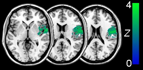
   The image below shows how changing a threshold can change the appearance of a statistical overlay. Consider the raw statitical map shown in the left panel, while the middle panel has been thresholded to only show voxels with Z-scores greater than 2.5 (with three regions surviving this threshold), the right panel shows a more conservative threshold of Z>4.5 - with only a single peak surviving.
   
5. We can repeat steps 2..4 to load multiple overlays, to compare different statistical tests. For example, clicking on the 'tutorialfmri.bat' icon will launch MRIcron and load to overlapping regions of interest. By using the Overlay/TransparencyOnOtherOverlays command we can view both of these overlays simultaneously.