Diffusion Tensor Imaging Analysis using FSL |
To complete this tutorial you will want the following:
This page describes Diffusion Tensor Imaging was written by Leigh Morrow, Paul Morgan and Chris Rorden. Diffusion imaging measures the random motion of water (and other liquids with hydrogen). DTI appears to be a tremendously important tool, as it is sensitive to acute brain injury (you can see strokes that can not be detected by conventional MRI) and it correlates with white matter integrity. Furthermore, in theory DTI values should be relatively calibrated - healthy adults should show similar values regardless of which scanner is used. This means that one can compare results to different atlases from other centers, for example the Hokkaido University Fractional Anisotropy Database. However, in practice different sequences can give dramatically different results (especially in terms of regional variability) so you probably want to use existing databases primarily as a starting point for developing a set of templates based on your own population, scanner and protocol.
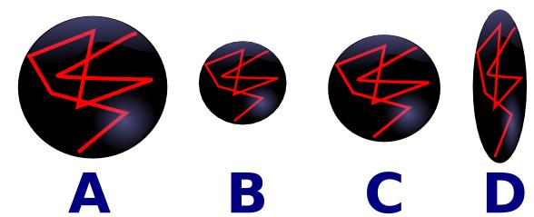
Furthermore, analysis methods for DTI remain primitive. Consider the drawing A below, where the red line shows the typical diffusion of a water molecule, randomly moving around - the black ball shows this molecules diffusion speed and direction. In constricted regions (e.g. inside cells) water is constrained, and the mean diffusion (apparent diffusion coefficient, or ADC) is slow, while in regions such as the ventricles the motion of the cerebral spinal fluid is unconstrained and relatively fast. For example, in the figure below, water is diffusing faster in A than B. On the other hand, in some areas such as along the fiber bundles of neurons (e.g. the brain's white matter) the diffusion properties are anisotropic - water will move in the direction of the fibers much more rapidly than orthogonal to the fibers. For example, in figure C below the water is moving isotropically, while in D the water is moving anisotropically. Therefore, are two ways to describe and analyze diffusion data. One is to describe it as having normal or abnormal ADC values per pixel (e.g. comparing A versus B). The other is to use the data for tractography to illustrate the shape and direction of fiber tracts (comparing C versus D).
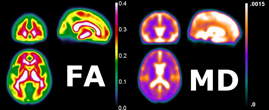
The figure below shows the fractional anistropy and mean diffisuity of a group of healthy individuals. Note that the FA is extreme in regions of white matter (e.g. the tensors look like Figure D above), while the gray matter is more isotropic (i.e. the tissue looks like figure C above). The MD map shows that the ventricles have high diffisuity (looking like Figure A above) while the gray and white matter have lower diffisuity (looking like B above).
You can view the raw DICOM files by dragging and dropping them onto MRIcron (or MRIcron's icon in the dock, if you use OSX). You can see that each gradient direction is acquired for each slice. There are multiple volumes, but each at a different diffusion direction. More diffusion yields a darker pixel because you lose signal as the water molecule can go anywhere. Higher ADC values mean it can go very far without interruption, and it takes the signal with it. This is not related to anisotropy.
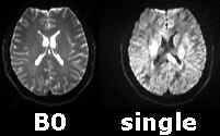
Below are some raw images from our DTI scan collected with our 3-Tesla Siemens Trio. On the left is the image for the mean B0 image which is not sensitive to diffusion direction. On the right is a single direction of the diffusion - note that the brightness varies dramatically in the white matter depending on the alignment of the fibers. More diffusion yields a darker pixel because you lose signal as the water molecule can go anywhere. Higher ADC values mean it can go very far without interruption, and it takes the signal with it. This is not necessarily related to anisotropy.
When the ADC values are calculated, they are done so in one direction at a time. It will repeat in different directions (different gradients) around a single point (the pixel). When you are in line with the pathways, you get a high diffusion value because it can move without being hindered. This results in a loss of signal (because it keeps going and going), and the image in that pixel looks dark. If the diffusion value is low, it is because the molecules are blocked by something else. Here, the image will appear bright.
In DTI, you use a tensor rather than a vector. A tensor is arranged as a matrix. You can split the tensor into 3 diffusion directions at right angles to each other. This will give you the eigenvectors and eigenvalues. There are 3 eigenvectors in each direction: the x, y, and z planes; however, we don’t know which eigenvector corresponds to which direction. The eigenvalues are used to determine which eigenvector corresponds to which direction. A high eigenvalue indicates that it is moving along with the fibers.
The more directions you collect, the better the image, but you also increase the risk of noise. One can increase signal by collecting more directions (e.g. 32 instead of 16) or increasing the number of times each direction is sampled (e.g. measuring 12 directions twice, and computing the average). However, additional directions or samples does increase the acquisition time, and people may move their head if they are scanned for extended periods. The minimum number of directions/gradients required to calculate the tensor is 6. More will give you a better estimation of the tensor (therefore better eigenvectors and thus better estimation of fiber directions). Approximately 15 to 20 directions is good, and will take about 5-minutes. But in tractography, you would say the more the merrier to get the better image.
You will also need to acquire a reference image with no diffusion information to calculate the ADC value (divide diffusion scan by reference scan). You can vary the amount of diffusion weighting (level of sensitivity to diffusion). The amount of diffusion weighting is measured by the b-value. If the b-value equals 0, there is no diffusion weighting (reference scan). If the diffusion value is very high, you can get greater resolution, but also more noise. The standard b-value for adults is 1000. In children, you typically use 600. If looking outside the brain, typically around 500.
Philips scanners will add an extra volume at the end of all volumes collected that shows the average of other diffusion scans. We don’t really want it, but it’s there anyway. It will always be the last one. For your convenience, dcm2nii will create two NIfTI images when you convert Philips DTI data: one with this ADC volume and another without this last volume
The sample dataset if already converted to NIfTI format and includes the b-values and gradient idrections. Often, we need to convert the images from a format used by the scanners (DICOM or PAR/REC) to a format that can be processed by FSL (Analyze NIfTI). The Siemens scanner only exports DICOM images. The Philips scanners can export data as either PAR/REC or DICOM. DICOM export is recommended, as getting the diffusion directions from PAR/REC is troublesome. A list of programs that can convert images from a scanner to the NIfTI format that FSL requires can be found here. However, it is important to note that you also need to extract the gradient direction and b-values as a text file. MRIconvert and dcm2nii can both create these files for you - in this tutorial I assume you have these files saved as DTI30s010.bval and DTI30s010.bvec
FSL has written the results as NIfTI format files, and you can open then in FSLView.
Your files should be saved in your data folder. It will save one file with the title 'FA', which refers to the Fractional Anistropy map. It also saves the three orthogonal vectors (V1, V2, V3).
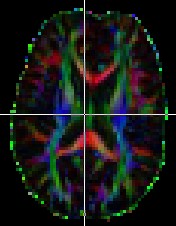
In FSL View, you can scroll at each axis, move crosshairs (+), move stuff with hand, and zoom with big box/little box, just click and drag. You can add lots of files as overlays. The L1, 2, and 3 are your eigenvalues, MD is the ADC value (mean diffusivity), and your eigenvectors are V1, 2, and 3 (along and perpendicular to filter if present). If you zoom in, you can see the direction with the slashes. You really only care about where its brighter/higher anisotropy).
The typical display seen in papers has the colors.
Here are a couple of additional tools for DTI processing.