MRIcro tutorial

This guide gives is a brief description of how you can use MRIcro and SPM to work with patient scans. For the MRIcro manual and software, visit the MRIcro home page (also available at www.icn.ucl.ac.uk/groups/jd/mricro/mricro.html). I also keep a have a FAQ that describes some of the more unusual features of MRIcro. Information about SPM can be found at www.fil.ion.bpmf.ac.uk/spm/, or at www.mrc-cbu.cam.ac.uk/Imaging/. This tutorial will describe the following features:

1. Download this tutorial
2. Viewing images
3. Creating regions of interest (marking and viewing lesions)
4. Segmenting a region of interest
5. Linear and nonlinear normalization functions
6. Normalize paitent scans in stereotactic space (SPM5)
7. Normalize paitent scans in stereotactic space (SPM2)
8. Normalizing patient (or EPI) scans in stereotactic space ( SPM99 )
9. Normalizing patient scans in stereotactic space ( SPMwin )
10. Creating multislice images
11. Creating multiple slices that only show one hemisphere
12. Working with multiple regions of interest
13. Yoking images to check registration
14. Displaying a rendered image of the brain's surface
15. Batch processing scanner images

Downloading this tutorial

• Windows users can download this tutorial by downloading the Windows installer.
• Linux users can download a zip file: shift+click here. This will copy a compressed version of the MRIcro web pages ('mritut.zip') to your computer (The zipped file requires around 450 kb).
• The MRIcro installation include a 1x1x1mm MRI scan. This is useful for learning how to use MRIcro. The image is named 'ch2bet.img': this is scalp-stripped version of the average of 27 T1-weighted scans of the same individual as displayed at www.bic.mni.mcgill.ca/cgi/icbm_view). A version of this image with the scalp included is also included with the latest MRIcro releases (this file is named ch2.img). Note that this MNI image does not exactly match the Talairach atlas. However, an MNI atlas is available.

Viewing an image

1. Select 'Open Analyze Format hdr+img...' from the 'File' menu. You will be asked to select the MRI you wish to view. At the Medical Research Council, the (normalized) T1 scans have the name 'n'+scan number (e.g. n12345) while the T2 ('pathological') scans have the name 'p'+ scan number (e.g. p12345).
2. The 'slice viewer' panel has three sliders: the top slider determines the scan slice you will be shown.
   

   Left: The 'Slice viewer panel'. Controls on this panel allow you to adjust the appearance of the image you have opened.

3. You can use the 'black' and 'white' sliders to adjust the brightness of the image. An automated brightness can be selected by selecting 'Contrast autobalance' from the 'View' menu. With some images (those with more than 256 levels of gray), adjusting the brightness sliders will cause the 'optimise contrast' button to appear (in the figure above, it is the black and white circle). Selecting 'Contrast autobalance' from the 'View' menu usually improves the image's appearance.
4. The bottom of the slice viewer panel allows you to select the cut you wish to view (transverse, sagittal, coronal, projection, free rotate or multiple slice views are available).
5. An easy way to view an image is to select the projection view, and then click on the brain image to select the coordinates you wish to view.

Creating a region of interest

1. Run MRIcro and select 'Open Analyze Format hdr+img...' from the 'File' menu. Enter the name and path of the file you wish to view.
2. You will probably only want to create a region of interest on the T1 weighted scan, but you may want to open up a T2/proton density/T2* image to check the lesion location. For more information on different types of MRI scans, visit Joseph P. Hornak's The Basics of MRI web page. The Whole Brain Atlas also has examples of MRI/CT data.
   

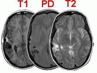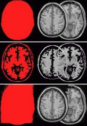
   Left: T1, proton density and T2 weighted slices from the same patient. The 'pathological' T2 scan is useful for locating the lesioned region in the brain. The 'anatomical' T1 scans usually have the best scan resolution, and are useful for localizing anatomical structures. The PD scan shows overall hydrogen density per cubic mm. Note artifacts caused by an aneurysm clip located directly anterior to the lesion (black hole, with a white halo in these images).

   Right: Relative brightness levels for different material in T1 and T2 scans. Notice that lesions are generally bright in T2 scans.

3. Regions of interest can only be drawn on the transverse, coronal and sagittal slices of the images (MRIcro versions prior to 1.20 only allow ROIs to be defined on the transverse slices). In the slice viewer panel, click on the button that shows a minature axial view of the brain. If the image does not appear to be sliced axially when the transverse button is selected (e.g. the scan looks coronal), then you may want to rotate the image, as described in the next section.
4. Press F3 to select the closed pen (or click on this tool in the region of interest panel).
   

   Left: Drawing a region of interest on a scan.

5. Go to the slice you wish to edit (you can use the F1 and F2 keys to go to the next lower or higher slice, respectively)
6. Draw the region of interest by dragging the mouse cursor around the border while depressing the left mouse button.
7. Go to the center of the region, an click the right mouse button to fill the region.
8. If you make a mistake, press the icon of the hand holding an upside down pencil (it is in the region of interest panel). This will erase your region of interest from this slice only. You can also shift-click to delete a region of a ROI. For example, shift-left-clicking deletes a region of interest beneath the mouse's movements, while shift-right clicking deletes a filled-region underneath the mouse's position.
9. Repeat steps 5-8 until you have drawn the lesion on all of the slices.
10. Choose 'Save ROI...' from the 'ROI' menu. It is often useful to give the ROI the same name as the image file (e.g. if the image file is n12345.img then the roi should be as n12345.roi).
11. Open the next image you wish to view. Repeat until you have created region of interest information for all of the images you want to process.

Note: MRIcro 1.36 and later includes tools for creating intensity-defined 3D regions of interest.

Segmenting a region of interest 

MRIcro can also be used to filter a region of interest based on the image intensity of the scan. For example, consider an fMRI study of auditory cortex. The experimenter has drawn a region of interest to delineate this region of the cortex, but is specifically interested if the activity of the gray matter is modulated with the task. To solve this problem, the experimenter could filter the ROI of auditory cortex in order to remove white matter from the analysis. Note that SPM99 has a series of sophisticated segmenting algorithms that may be more accurate than MRIcro in many instances. MRIcro can apply an intensity filter to the entire volume (so the same contrast levels are applied to all of the slices in the entire image), to a single slice or to a region within a single slice.

Here is a step-by-step guide for segmenting an ROI using MRIcro:

1. Draw your ROI as described in the previous section.
2. Make sure to adjust the contrast of your image so that the different tissues appear visually distinctive. For images with more than 8 bits per voxel you may want to use the precision contrast tool (select 'Precise contrast' from the 'Viewer' menu).
3. Select 'Apply intensity filter to slice/region...' from the 'ROI' menu. You will then be asked if you want to apply the contrast filter to the entire slice or a region of the slice. If you want to apply the filter to only a region, you will be asked to click on the top-left and bottom-right corners of the region you wish to filter. In the example below, we want to apply a different threshold to the dark clip artifact than the bright lesion. Therefore, we need to select the appropriate region.
4. Adjust the intensity thresholds so that the tissue you want to preserve is highlighted in green. For example, when selecting the gray matter, the image might look like the panel C in the figure below.
5. Press the 'Filter as shown' button.
6. If you plan to use the ROI with SPM, you will want to convert the ROI to an Analyze format image. To do this, choose 'Export ROI as Analyze image...' from the 'ROI' menu.

Linear and nonlinear normalization functions 

SPM can be used to 'normalize' MRI scans. These functions reorient the angle, position, size, etc of the scan to standard stereotaxic space. Normalized brains are much easier to read, because the slices match those available in published atlases. In addition, the majority of modern functional imaging studies normalize their scans to standardized space. Therefore, if you normalize your patient scans, the resulting scans will be easy to interpret relative to each other, to atlases and to functional imaging studies. However, SPM's normalization routines can be disrupted by a patient's lesions. This is because the lesioned region is very different from the corresponding region in the template (that comes from a healthy individual). In particular, SPM's non-linear routines are sensitive to lesions, and these routines will try to eliminate the lesion by compressing that region (distorting the shape of the brain in the process, see the figure below). There are two solutions. First, you can normalize the brain using only the linear components of the coregistration (e.g. set the parameter estimation defaults so that there are no nonlinear iterations and no basis functions). This method tends to do a fairly decent job of coregistering the brain. If you are using SPM99, you can take advantage of its 'object masking' feature to coregister a patient's scans. With this method, the masked region (e.g. area of a lesion) does not influence the parameter estimation. The advantage of this method is that SPM can apply nonlinear basis functions to the image, allowing a better coregistration. In addition, the lesion does not influence the linear components of the normalization, allowing a better linear fit as well. This section describes how to implement this technique.

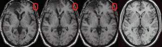Left: Linear, linear+nonlinear, and masked linear+nonlinear (respectively) normalizations of the same image to the MNI representative brain (shown on the far right). Note that without a mask (2nd from left), the nonlinear components compress the lesion, hiding the true position and size of the lesion. This example is from Matthew Brett.

The table below shows each of the linear functions (translation, rotation, zoom and shear) applied to representative input images. Note that all of these functions can be applied in each of the three dimensions (e.g. rotation can be applied in the x, y and z coordinates, correcting yaw, pitch and roll of the input image). With the linear functions, note that any three points that are colinear in the input image will also be colinear in the output (though two parallel lines in an input image may not be parallel after an affine transformation). Also, all of the 12 linear parameters (translation, zoom, rotation and affine functions each in the x,y and z dimensions) are computed based on information from the entire image -therefore these functions are rarely disrupted by unusual local features found in MRI scans (e.g. aneurysm clip artifacts or lesions). The final row in this table shows how a nonlinear basis function can be used to coregister a brain image. In the representative example, the input image has a fisheye effect, which can be compensated for by a simple basis function. Unlike the linear functions, points that are colinear in the input image may not necessarily be colinear after nonlinear normalization. Furthermore, nonlinear functions are more heavily influenced by local image information, and therefore nonlinear normalization of patient scans may lead to distortion due to the unusual appearance of the lesion or aneurysm clips. For this reason, it is important to mask lesions and clip artifacts when estimating a nonlinear normalization (see the next section, which describes lesion masking in SPM99).

Input	Function	Output
	translation (e.g. shift up) rigid body transform
	rotate (e.g. pitch down) rigid body transform
	zoom (e.g. stretch wider) affine transform
	shear affine transform
	nonlinear basis function (e.g. shrink middle, expand edges)

Normalize patient MRI scans with MRIcro and SPM5

Normalize patient MRI scans with MRIcro and SPM2

This section describes how to mask lesions so they do not disrupt the automated normalization functions of SPM2. Using this technique, SPM2 can accurately align a patient's scan to stereotaxic space without causing undue distortion. To complete this you will need SPM2 beta (or later) and MRIcro version 1.19 or later.

Stage 1: using MRIcro on a Windows PC:

1. Open the patients MRI scan and ensure that the scan is in the correct orientation and you have marked the anterior commissue (see Stage 1, steps 1-2 of the section on normalizing patient scans with SPM99).
2. Use MRIcro's Region of Interest tools to create a ROI that accurately maps the location and extent of the lesion (see the earlier section on creating ROIs).
3. Make a lesion image. With your image and ROI open, choose 'Export ROI as Analyze image...' from the 'ROI' menu.Choose 'ROI is 1, background is 0' and save the image with the prefix 'l' (for 'Lesion', so if your file is named 'filename.img', you will have a new image named 'lfilename.img'.
4. Make a masking image. With your image and ROI open, choose 'Export ROI as smoothed Analyze image...'. Choose a FWHM smooth of 8mm, a 0.001% threshold and make sure you select 'ROI is 0 [SPM object mask]'. Save your image with the prefix 'm' for mask. So if your original filename was 'filename.img', the mask image should be 'mfilename.img'.

Stage 2: using SPM2 to normalize your image:

Note: you will want to have the file 'lesionmask.m' in the same folder as SPM2. This simple script will allow you to quickly normalize images with SPM2. You may want to read through this script to ensure that it is accurate for your images: it assumes you are converting T1-weighted images. In addition, it is assumed that you have 3 Analyze files for each individual, all in the same folder: 'filename.img', 'lfilename.img', 'mfilename.img'. These files represent the MRI scan, the lesion definition and a smoothed version of the image that is used as a mask.

1. Open Matlab and type 'lesionmask' into the command window.
2. You will be asked to select your images. Only select the MRI scans (e.g. filename.img), you should not select the mask (mfilename.img) and lesion (lfilename.img) images. Note you can select multiple files to batch convert images.
3. SPM2 will then normalize images, the output will be a normalized version of the MRI scan ('wfilename.img') and a normalized copy of the lesion ('wlfilename.img').

Stage 3: using MRIcro on a Windows PC:

1. Save the lesion in MRIcro's compressed ROI format. Open the lesion defintion scan (e.g. 'wlfilename.img') select 'Export Analyze image as ROI...' ('ROI' menu). You will be asked to set a minimum threshold for accepting a region as a lesion: you should set this value to 50 (50% of the maximum image intensity). Give this the same name as the patients normalized image (the ROI for image 'wfilename.img' should be 'wfilename.roi'.
2. Open the normalized patient image with the 'Open image...' command ('File' menu). This should load both the normalized image and (if you have successfully completed the previous step) the normalized ROI. Notice that the volume of the lesion is displayed in the region of interest panel. Make sure to save your ROI. You can now view the lesion from any view and get a good idea of the size/position of the lesion (all in standardized stereotactic space).

Normalize patient MRI scans with MRIcro and SPM99

This section describes how to mask lesions so they do not disrupt the automated normalization functions of SPM. This technique is also useful for EPI fMRI images from healthy individuals (where EPI artifacts can also disrupt normalization). The MRC-CBU has a page devoted to EPI masking. Souheil J. Inati has also posted a useful technique for normalizing EPI scans with SPM.

SPM99 can compute normalize patient scans to a stereotaxi standard template using both linear and nonlinear functions. Allowing SPM to apply nonlinear transformations will generally result in a more accurate normalization. However, with patient scans, nonlinear functions can effectively squash the region of a lesion (as it has no equivalent in the healthy template brain), causing considerable distortion of the brain. This section describes how to create and apply a lesion mask with SPM99, which allows accurate linear and nonlinear normalization of scans that have large lesions.

You will require SPM 99 beta (or later) and MRIcro version 1.19 or later (to get the latest version of MRIcro, go to the MRIcro home page).

Stage 1: using MRIcro on a Windows PC:

1. Open your scan and check the image orientation and the amount of neck presented in the image: when the slice viewer panel is set to display transverse slices, you should see transverse slices with the anterior portion of the brain (and the nose) toward the top of the screen and the posterior regions of the brain toward the bottom of your computer screen. Furthermore, the amount of neck displayed in your image should roughly match the amount of spinal cord shown in the template image. If your image is not in the correct format, choose the 'Save as...[rotate/format/clip/4D->3D]' from the 'File' menu. A window will appear which allows you to describe the current orientation of the brain and the amount of the spinal cord you wish to clip from the image. The preview button allows you to ensure that you have selected the correct orientation. Once you have correctly described the image orientation, press the 'save Intel' (or 'Save Sun', both SPMwin and MRIcro can read either format). Advanced note: if all of your scans are in the same non-transverse format (e.g. coronal), you can set SPM96/SPM99 [but not SPMwin] to automatically rotate the scans for you by setting the 'sptl_Ornt' parameter of your spm_defaults.m file. For more details, search the SPM archives for 'sptl_Ornt'. Another option is to reorient the images using SPM99's 'display' feature.
   

   Left: The left panel shows a coronal format scan. Note that when the transverse view button (highlighted in green) is selected, the scan appears to be coronal. The right panel shows MRIcro's scan rotation panel, with the format for the scan set to coronal. Note that the rotation panel has 'clip low' and 'clip high' settings, which allow you to interactively shave slices off of the image. In this example, I want to remove some of the excess spinal cord, so that this region will not influcence SPM. Note that the sagittal view on the right shows much more spinal cord than the template brain (shown in the projection view, below).

2. Make sure that the 'origin' fields correctly designates the location of the Anterior Commissure (see the diagrams below to get an idea of where the AC is located, or read Matthew Brett's AC-PC web page). To find the AC, click on the projection views button (it looks like a cube) and make sure that the 'XBars' command is selected. Then, use the mouse to click on the location of the AC (in the example below, the AC is located near 46 64 37). Once the image cross-bars are positioned at the AC, input the X Y and Z coordinates listed in the 'slice viewer' panel into the origin fields of the 'header information' panel. You should then save the header (press the floppy disk icon located in the header information panel).
   

   Left: The location of the anterior commissure (AC) on the Montreal Neurological Institute's representative brain. The location of the crossbars (which are now at the AC) is given at the top of the slice viewer panel (lower left) . These values should be placed in the 'Origin' fields (upper left) of the header information panel in order to tell SPM the location of the AC.

3. Making the lesion definition image. Open the source image with MRIcro and create a region of interest (see the earlier section on creating ROIs) that includes the region of the lesion only. Using MRIcro's 'Save ROI as Analyze image...' command (from the 'ROI' menu) to convert the lesion into a format that SPM can read. As a convention, I usually add the 'L' prefix to these lesion definition files, so the lesion for image '123.img' should be 'L123.img'. Advanced note: If you draw the lesion in one plane only (e.g. drawing on transverse slices only) your ROI will usually have discontinuous stepping artifacts in the the dimension orthogonal to the plane you are drawing in (e.g. when drawing the ROI on transverse scans, you are marking images in the X and Y dimensions, and the Z dimension may having stepping artifacts). These irregularities will look unusual when SPM normalizes the lesion into stereotaxic space. One solution is to use MRIcro to save smooth the lesion before normalization. To do this, choose the 'Export ROI as smoothed Analyze image' function [instead of the unsmoothed function] and select a narrow smoothing band [4mm] will a 50% cutoff [Threshold=0.5], and make sure that the dropdown box selects 'ROI is 1 [reslice ROI]. Press save, and give the file a suitable filename for a lesion definition (e.g. my convention is to add the 'L' prefix to the file name). Saving the lesion definition with these smoothing values will create an image file that is no larger than the original lesion but does not have any specific stepping artifacts.
4. Make the mask image -if the MRI scan includes any regions of unusual appearance besides the lesion (e.g. any clip artifacts), add these to your MRIcro ROI. Essentially, you want to mask out any unusual regions of the brain that do not have an equivalent on the template image and therefore can throw off SPM's normalization routines. Then save this as an image mask by choosing the 'Export ROI as smoothed Analyze image' function. This will save the region of interest as an Analyze format image. You will use this as the mask in SPM. As a convention, I usually add the 'm' prefix to these mask files, so the mask for image '123.img' should be 'm123.img'. Advanced note: This window has a number of options for controlling the amount of smoothing, the full width half maximum (FWHM) describes the width of the smoothing function, which should be the same as you are using in SPM (often 8mm). The threshold sets the mask's sensitivity to the presence of an ROI: 0.001 is standard. In addition, you can set how the filter deals with the edge of an image -you will probably want to keep the setting at 'Adjust sides in Z-plane only [SPM]', which precisely mimics SPM's behavior (and will show the same edge boundary artifacts as SPM). Finally, make sure that the final drop down box is set for 'ROI is 0 [SPM object mask].

Stage 2: Using SPM99 on a UNIX machine or with Windows NT:

1. Launch SPM99. This will vary depending on your system, usually you start Matlab and then type 'SPM' in the Matlab command window.
2. Press the 'PET/SPECT' button (or the 'fMRI' button, it does not matter for image normalization).
3. Check the settings by pressing the 'Defaults' button and choosing "defaults/spatial normalization/parameter estimation"to make sure that the "masked object brain"setting is set to "true".
4. Use the 'Display' button to check that the image horizontal plane is roughly that of the AC-PC line (see the figure above, you may need to adjust the 'pitch' setting). If you change the image orientation, make sure to save the settings by pressing 'reorient images'.
5. You are now ready to normalize the images.Press the 'Normalize' button and choose the 'Determine parameters and write normalized"function.
6. You will be asked to locate four sets of images:
   • The image you wish to get the parameters from (the patient's scan, e.g. 123.hdr)
   • The mask file (e.g. the mask you made from the patients ROI file, e.g. m123.hdr).
   • The images you wish to write these parameters to
     -the patient's scan (e.g. 123.hdr)
     -the lesion definition file (e.g. L123.hdr)
   • The template image (e.g. look in SPM's template folder and choose T1.img)
7. SPM will now normalize your brain. The output files will be named with the prefix 'n' (e.g. if your patient's brain is 123.hdr', the output will be 'n123.hdr', and if the lesion definition is 'L123.hdr', the output will be 'nL123.hdr').

Stage 3: using MRIcro on a Windows PC:

1. Save the lesion in MRIcro's compressed ROI format. Open the lesion defintion scan (e.g. 'nL123.hdr') select 'Export Analyze image as ROI...' ('ROI' menu). You will be asked to set a threshold for accepting a region as a lesion: you should set this value to 50 (50% of the maximum image intensity). Give this the same name as the patients normalized image (the ROI for image 'n123.hdr' should be 'n123.roi'.
2. Open the normalized patient image with 'Open Analyze format .hdr + .img' ('File' menu). This should load both the normalized image and (if you have successfully completed the previous step) the normalized ROI. Notice that the volume of the lesion is displayed in the region of interest panel. Make sure to save your ROI. You can now view the lesion from any view and get a good idea of the size/position of the lesion (all in standardized stereotactic space).

Normalize patient MRI scans with MRIcro and SPMwin

SPM for windows (SPMwin) is a freely available standalone implementation of SPM96. Unlike other versions of SPM, SPMwin does not require Matlab. Therefore the software is completely free and many users find the user interface friendlier than Matlab versions of SPM. However, the current release of SPMwin does not implement SPM99's ability to create object masks for normalization of patient scans (see the previous section for details). However, for the majority of patient scans, SPMwin can do a reasonable job of coregistration, with the caveat that the normalization should only include linear transformations. The nonlinear transformations will often distort patient scans in an attempt to eliminate the region of the lesion. See the section on linear and nonlinear transformationsfor more details on the advantages and disadvantages of applying nonlinear transformations to patient scans.

You will require SPMwin and MRIcro version 1.19 or later (to get the latest version of MRIcro, go to the MRIcro home page)

Stage 1: using MRIcro on a Windows PC:

1. Open your scan and check the image orientation and the amount of neck presented in the image. The previous section explains this step in detail .
2. Make sure that the 'origin' fields correctly designate the location of the Anterior Commissure. The previous section explains this step in detail .

Stage 2: Using SPMwin on a Windows PC:

1. Run SPMwin. From the 'File' menu choose the 'new/normalization' command. Once you have told the computer how many scans you wish to normalize, you will see a window named 'spatial normalization' with the icon of a small book. Double click on the icon, you will see four small icons labelled 'template','image to estimate parameters' and 'image to normalize'.
2. Double click on the template icon. Make sure that the listed template is the correct one for your patient's scan (e.g. if you are normalizing a T1 scan, make sure that the template is 'T1.hdr'). If it is incorrect, click on the filename and press delete, then drag and drop the correct template header to SPMwin's template icon.
3. Drag and drop the patient scan's header file to both the 'image to estimate parameters' and 'image to normalize' icons.
4. You may want to check the settings by choosing the 'settings' command from the 'calculate' menu. If so, make sure that 'sync' interpolation is selected in the 'general' tab. Makesure that the 'Number of nonlinear iterations' and 'Number of basis functions' are both set to zero (parameter estimation tab). Also check the reslicing dimensions in the 'reslicing' tab.
5. Choose 'start' from the calculate menu. When the normalization is complete a new image file will be created, which will have the prefix 'n' (e.g. if your patient's scan had the name '12345.img', the normalized scan will be named 'n12345.img').

Stage 3: using MRIcro on a Windows PC:

1. Open the normalized scan (e.g. n12345.vhd and n12345.img). Press the floppy disk icon in the header informtion window to create an Analyze format header (n12345.hdr).
2. Create region of interest that marks the region of the lesion (as described in the 'Create ROI' section). This region of interest should only include the regions of the lesion. Notice that the volume of the lesion is displayed in the region of interest panel. Make sure to save your ROI. You can now view the lesion from any view and get a good idea of the size/position of the lesion (all in standardized stereotactic space).

Creating multislice views

MRIcro allows you to quickly create 'multislice' images that show a number of preselected cuts from an scan. This can be useful for presenting similar slices from a number of patients. This section describes how to generate a multislice view.

1. Open the image you wish to view by choosing "Open analyze format hdr+img". If you want to superimpose a region of interest [ROI, e.g. an outline of a lesion] there are two options. First, if the ROI has the same name as your image (e.g. the image is named "mr1.img" and the ROI is "mr1.roi", the ROI will have been opened automatically when you loaded the image. If the ROI has a different name, or if you want to superimpose multiple ROIs, select "Open ROIs..." from the 'ROI' menu. A dialog box will appear and you can control+click on each ROI you wish to open [e.g. for the tutorial, you can open "a.roi","b.roi" and "c.roi" simultaneously].
2. Open the Etc menu's 'Option' window and select the slices that you want to view (these values are shown outlined by yellow in the figure below). You can display up to twelve slices, but if you wish to show fewer slices enter a zero into the unused fields. For this stage you must enter the slice number rather than the Talairach position (e.g. in the image that comes with this tutorial, Z of 0mm is on the 37th slice, so to show Z=0mm enter the number 37). An easy way to find the corresponding slice number is to show the projection view of an image. You can then adjust the slice number (using the boxes in the slice viewer panel) and see the corresponding Talairach coordinate (if the slice viewer's 'info' button is selected).
   
3. I typically display axial slices 48, 56, 64, 72, 80, 88, 96, 104, 112, 122, and 132 (for normalized images with 1mm slices, like the image that is downloaded with this tutorial). These slices correspond to Talairach slices -24, -16, -8, 0, 8, 16, 24, 32, 40, 50, 60mm, which are common transverse slices.
4. The options window has a number of additional settings that control the multislice view. Once you have selected your desired settings, press the 'OK' button. (MRIcro will remember your preferred settings, so you usually only have to set these up once). There are a number of options that you can choose:
   • Select whether you want to view Transverse or Coronal slices. I usually show tranverse views, but for some images (e.g. showing hippocampal lesions), the coronal view may be more appropriate.
   • Select whether you want to see a sagittal view.
   • Select from the various options for the sagittal view.
5. To generate a multislice view, click the multislice view in the Slice Viewer panel. You should see a multislice image similar to the one displayed below.
   

Creating multiple slices that only show one hemisphere

Recent versions of MRIcro have made this a bit easier and more powerful. This tutorial describes features in MRIcro 1.35 and later.

1. Select 'Open Analyze Format hdr+img...' from the 'File' menu. You will be asked to select the MRI you wish to view.
2. Open the Etc menu's 'Option' window and make sure that multislice options are set for 'Show right hemisphere' (this box is outlined in green in the diagram of the Options window shown in the previous section) , or 'Show left hemisphere' if you wish to show the left hemisphere. You can also set the other multislice options by setting the approriate check boxes and values.
3. Set how whether you want to see coronal or transverse slices, and set how much overlap you want: you can values between 1/2 (the entire left side will be hidden) to 1/5 (only a small chunk of the left side will be hidden. These controls are outlined in red in the diagram of the Options window shown in the previous section)
4. Press the 'Set Mask' button to interactively adjust the border threshold (also outlined in red in the diagram of the Options window shown in the previous section). A dialog box appears that allows you to set the boundary threshold for your image. As you adjust the threshold image, portions of your image that are above the threshold will appear as the region of interest colour (red in the left images on the figure below) . Adjust the threshold so that the skull defines a boundary for the brain (top panel in the image below) .If the threshold is set too high (middle panel below) or too low (bottom panel below) , the resulting multislice will show mask artifacts (the right side of each panel shows the corresponding multislice for each mask setting).
   
5. When you are happy with your settings, close the threshold window and close the Options window.
6. Press the multislice button in the slice viewer panel (it has an icon with multiple brain images).
7. If you are happy with the result, you can use the 'Save as picture' command to save the image in a standard graphic format of your choice.
8. WARNING : If you have set the 'translucent ROIs' checkbox in the Option window, you should ensure that all regions of interest exist only in the hemisphere that is to be displayed. Translucent regions of interest (and for advanced users, functional imaging hotspots) are added after MRIcro has overlaid the scans, and ROIs in the hidden hemifield can appear on the visible hemisphere of the incorrect slice.

Working with multiple ROIs

It is often useful to display overlapping regions of interest (ROIs) from different individuals. For example, after you have normalized the brain scans from several neurological patients, it can be useful to explore the regions of mutual involvement. There are a couple of important issues to bear in mind when combining multiple ROIs. First of all, all of the ROIs need to be from spatially coregistered images - i.e. the ROIs must have the same voxel size and image dimensions. Consider if we want to examine the ROIs from patients A and B. These two patients are shown in the picture below as 'A' and 'B'. The first thing we might want to generate is a density plot, that would should us which regions are mutually involved.This is represented as A+B in the figure below. To do this, you can conduct the following steps:

1. open a template image that has the same spatial dimensions as the patient's images.
2. Open the ROIs using the 'Open ROI[s]...' option from the ROI menu. Select multiple ROIs by control+clicking on the different filenames.
3. MRIcro now shows the overlayed lesions, as illustrated by A+B below.

However, it can also be useful to apply boolean (logical) operators to the ROIs. MRIcro includes three logical ROI operators - intersection, union and subtraction. Each of these commands is found in the "ROI comparisons" submenu of the "ROI" menu. For example, we could find the region that is involved in two groups of patients. In this case we could compute the INTERSECTION of the two data sets (a logical "AND"): Only voxels which are present in ALL the ROIs will be present in the output ROI. Another reasonable comparison would be to examine the UNION of two data sets (a logical "OR"): voxels present in ANY of the ROIs will be included in the output ROI (AUB in the figure above). A final useful comparison is MASK, where MRIcro identifies the region that is unique to A (AmB in the figure above). Note that in the sample above only two ROIs were compared. In practice, you can apply the comparisons to many ROIs simultaneously (control+click on the file names to select multiple ROIs).

Lesion density plots (A+B in the figure above) have become a common tool method for attempting to infer the functional role of an anatomical region. However, you should be careful with the inferences you draw from density plots. One problem is that the size and extent of naturally occurring lesions is typically determined by vasculature (for strokes), and susceptibility to sheer and impact (for traumatic brain injury) rather than function. Therefore, simply overlapping lesions from patients who show a specific deficit will often highlight regions involved with the function as well as regions that are simply more susceptible to damage. One potential solution is to directly compare patients with a specific deficit to control patients with a SUBTRACTION analysis. Regions that are susceptible to damage will be occur with similar frequency in both groups, and be effectively cancelled out. On the other hand, regions that are required for the target function will tend to be damaged in the target patients but not in the control patients. In any case, note that naturally occurring lesions vary greatly in the location and extent of the damage, adding a huge amount of variability into an analysis. This large variance substantially reduces the power of anatomical studies. One solution is to conduct analysis on a large number of patients. A second solution is to restrict analysis to patients with focal lesions.

The "ROI comparisons" submenu also allows you to compare SUBTRACTIONs between two different groups of patients. This allows you to identify if certain regions are more common for one pathology than another. To implement this command, you should first open your template image. Then choose the "Subtract ROIs" command. You will then be asked to select the positive ROIs. Next you will be asked to select the negative ROIs. The figure below illustrates two groups of patients (A and B). The right panels show the subtraction between these two groups (A-B, A-B%). You can either subtract the absolute numbers or relative percentages (the default setting). Select 'ROI density colorbar' from the ROI menu to see a legend. The percentage subtraction shows 11 levels of ROI: each bar represents 20% increments - so the lightest blue represents 81..100% B. The middle purple percentage bar designates regions where there is an identical percent of A and B (0%). Comparisons are most meaningful when both groups are the same size.

Yoking images to check registration

SPM99 includes a feature named 'check reg' that allows you to view the same Talairach coordinates for two Analyze format images. This function is useful for testing the normalization of scans to a template. MRIcro's yoking feature is conceptually identical, but allows you to check the coregistration of two or more images simultaneously. Viewing more than two images allows one to check the normalization of several images to a template, or to compare to different normalization techniques with each other.

To view yoked images, launch one copy of MRIcro for each image you wish to view. Load the images and make sure that the 'Yoke' checkbox is selected. Once this is done, the images will all show corresponding slices -irregardless if the images are sliced to different dimensions (e.g. one image shows 1mm slices, whil the other shows 2mm slices) or whether the images are cropped differently (e.g. one image showing more of the skull). To move to a different position, click on the desired location in any of the images -the other images will be updated to match your selection. It is generally useful to shrink the toolpanel and optimize the formsize (in the 'Viewer' menu) when viewing multiple images, allowing you to maximize the available screen space.

In the example below, three images are yoked simultaneously -showing (from left to right) a template image and the scans from two neurological patients. The two left most scans are from the same patient -notice that the nonlinear functions of the normalization have compressed the lesion in the rightmost scan (as described in the normalization section). Clicking on any position in any of the three scans will show the corresponding location in all three scans. Note that in this example the images are cropped differently -with the normalized images showing less of the skull than the template. Despite this, the yoking finds the corresponding location in all three images.

Displaying a rendered image of the brain's surface.

I now have a web page devoted to volume rendering with MRIcro.

Batch processing scanner images.

Note, there are new tools that can convert your images directly to NIfTI format. You can find a listing at my dcm2nii website

Most MRI systems export scans as in either DICOM or a proprietary format. Unfortunately, SPM and many scientific packages require Analyze format files. MRIcro can convert many common medical image formats to the Analyze format file. For a list of the formats supported by MRIcro and other free converters see MRIcro's home page.

This section describes how to stack a series of two dimensional images to create three dimensional volumes. Most fMRI studies will generate a vast number of scans, and MRIcro is designed to ease the conversion of these scans for processing with SPM or other brain imaging packages.

The batch processing panel is the most complicated feature of MRIcro for the user. Unfortunately, different scanners use very different methods for saving images. MRIcro has been designed to work in many different situations, and this flexibility has meant that the interface is rather complex. However, images from a single scanner are virtually always in the same general format, so once you have tuned MRIcro's conversion the first time, subsequent conversions should be simple.

As an example, consider a series of DICOM format file's named a11.dcm...a31.dcm that contain slices from two brain volumes. Each volume is composed of three slices. Furthermore, only every fourth is relevant (e.g. the other scans were not T1 images), so the relevant slices are image a11, a15, a19, a23, a27 and a31. In addition, the orientation of these scans does not correspond with the standard SPM axial slices.

The left column in the figure above shows the six DICOM images in this example. We will process the images in two steps. First, we will convert all of the slices to a single multivolume Analyze format image (that SPM can not use). Next, we will rotate the images to the correct orientation and convert each volume to a separate Analyze format file (that SPM can read).

Here is the sequence of steps to batch process these images:

1. Launch MRIcro and select 'Convert DICOM/Genesis/Interfile/Siemens/Picker to Analyze' from the 'Import' menu.
   
2. A new window appears (as shown above). For our example we will want to adjust the values to match our data set:
   • Number of files: Total number of slices to be converted (in our case, 6 slices).
   • Increment: what is the numerical spacing between successive images (in our case, this should be 4, as every fourth scan is the T1).
   • Volumes: How many brain volumes are we converting (in our example there are two brain volumes).
   • First file is dorsal: Select this to reverse the slice order (e.g. the slice order is dorsal to ventral). In our example, slice order is ventral to dorsal (the first slice [a11] is ventral), so we will leave this button unchecked.
   • Interleaved slices: Check this if the slices from the different volumes are interleaved, rather than sequential. In our example, the volumes are sequentially stored (the first slices [a11, a15, a19] belong to the first volume followed by the slices for the next volume [a23, a27, a31]). If the slices for the first volume were a11, a19, a27 and slices from the second volume were a15, a23, a31 we would want to select this checkbox.
   • Use extension as index: select this if the image index number is in the extension, e.g. a.11,a.15,...a.31. On our files, the extension (.dcm) is not the index, so we leave this option unchecked.
   • Sort Using DICOM index, not filename: Some scanners name slices based somewhat randomly (e.g. saving the files as file1.dcm, file6.dcm,file2.dcm,file5.dcm,file3.dcm,file4.dcm). These scanners often save the true sequence in the DICOM header (group/element 0020h/0013h). This option will reorder the slices based on information in the DICOM header. Our files are indexed correctly by the filename, so we can leave this unchecked.
   • Open sequential files: ignore filename: Unfortunately, some scanners save images with a very complicated file naming system that MRIcro will not be aware of (e.g. fileA-1,fileB-2,fileC-3,etc). In this case, I suggest that you write a simple program to rename the files to a numerical sequence that MRIcro can interpret (e.g. file1,file2,file3). However, as a last resort you can have MRIcro ignore the filename altogether and open sequential files in a folder. Important: Before using this option, place the image files you want to convert into a folder that has no other files of any type in it. This option may or may not work- your images may end up in a scrambled order. It works best best when used in conjunction with the "Sort Using DICOM Index" option. In our example, we will [thankfully] leave this option unchecked.
3. Press the 'Design' button to check that you have correctly described the slice order. A window appears that shows the slice order, indexed from one. In our example, the design window will list:
     Volume 1: 1, 5, 9
     Volume 2: 13, 17, 21
   This accurately describes our data with the first volume storing the 1st, 5th and 9th slices (a11, a15, a19) and the second volume storing the 13th, 17th and 21st slices (a23, a27, a31).
4. Once you have described the slices, choose 'Select' and find the first DICOM (or NEMA, Genesis) file in the series (i.e. the slice with the lowest numerical value, in our example this is a11.dcm). The file names must end with the numberical index (a11.dcm is valid, 11a.dcm is not). Optionally, the file index may be padded by zeros (e.g. file008.dcm, file009.dcm, file010.dcm is valid, as is file8.dcm, file9.dcm, file10.dcm).
5. Give a name for the output Analyze format image (e.g. lets call it 'out.img').
6. MRIcro should now process all of the slices and create a multivolume Analyze format image. If successful, you can close the DICOM conversion window.
7. You will now be able to open the image by selecting 'Open analyze img+hdr...' from the 'File' menu. You can only view volumes one at a time, so MRIcro will ask you to name the volume you want to view.
8. You should now check the header information panel and make sure all of the information is correct.

   • You may want to adjust the image intensity value shown in the header information panel. SPM will use this scale for determining the signal level. This is especially crucial for SPM99b (the final release of SPM99 should do this automatically). See the SPM99 normalization section of this tutorial for details on how to automatically adjust the image intensity.
   • Check to make sure that the slice thickness (Z size [mm]) is correct.

9. To extract the individual brain volumes, select 'Save as...' from the 'File' menu. A new window appears. You may want to adjust the orientation by selecting the 'format' and checking the results with the preview. In my example, the images need to be rotated 180 degrees in the Z plane, so the format needs to be set to 'axial down'. Click the 'Save Intel' button to extract and rotate all of the volumes. You will be asked to give the output a name, for example if you name the output 'xout.img', the files will be called 'xout1.img', 'xout2.img'...etc.
10. You can now delete the multivolume image if you wish (in our example, out.img).

In our example, each DICOM file contained one image. Furthermore, the two volumes were stored sequentially rather than being stored with 'interleaved slices' (that is, all the slices for the first volume had lower numbers than the scans for the second volume). Note that the design window allows you to adjust these features.

Interleaving: In the figure on the left, slice interleaving is shown on the right panel. In our example, the volumes were saved sequentially (e.g. all of the first volume's slices had lower indexes [a11, a15,a19] than the second volume [a23, a27, a31]). However, some scanners save volumes in an 'interleaved' format. Selecting the 'slice interleaving' option will tell MRIcro that the slices are interleaved (e.g. the first volume is a11, a19, a27, and the second volume is a15, a23, a31).

Mosaics: The NEMA format only specifies image size in two dimensions, so 3D volumes are stored as 'mosaics', which show various cuts on the same plane. The figure aboveshows a 2x3 NEMA mosaic. One way to test whether your images are a mosaic is to select 'Open foreign' from the 'Import' menu. If you see multiple slices simultaneously, you are dealing with a mosaic. MRIcro should automatically detect and convert Siemens images if you click the 'Autodetect Mosaics' checkbox (though see Interleave note below). Otherwise, you will have to manually set the mosaic height and width when converting the images to Analyze format. Note that the more recent DICOM format does describe images in three dimensions, so quick opening these files will show only one slice per plane (and for conversion purposes, you should set the mosaic height/width both to 1).

Interleaved Mosaics: Most mosaic files store slices in the same order we read English: starting from the top left and reading from left to right. However, some Siemens scanners create mosaics where the slice order is interleaved within the mosaic. If you select 'mosaic slice interleave', MRIcro will try to correctly read the order of Siemens mosaics. Note that the 'Autodetect Mosaics' checkbox will NOT detect slice interleaving for Siemens Vision mosaics, as some fMRI labs have created and distributed acquisition protocols that incorrectly set up the image header. Therefore, Vision users must always manually determine if the mosaic images are interleaved.